Benford’s Law after converting count data to be in base 5

Firstly, I know nothing about election fraud – this isn’t a serious post. But, I do like to do some simple coding. Ben Goldacre posted on using Benford’s Law to look for evidence of Russian election fraud. Then Richie Cotton did the same, but using R. Commenters on both sites suggested that as the data didn’t span a large order of magnitude, turning it into a lower base (e.g. base 5) may helpful. I’ve no idea if this would be helpful, but the idea of messing around with the data was appealing, so here it is.

The as.binary() function was posted to R-help by Robin Hankin. The code to do the analysis was by Richie Cotton. Putting it all together gives:

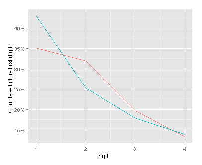
So there we have it – with the numerical data in base 5, the observed and expected values are closer together than with the numerical data in base 10. The overall dynamic range is from 1 to 30430 (in base 5).

The data are here. The code you’ll need is:-

 
## repeat the analysis but with base 5
rm(list = ls())
library(reshape)
library(stringr)
library(ggplot2)
russian <- read.csv("Russian observed results - FullData.csv")

as.binary <- function(n,base=2 , r=FALSE){ 
  ## function written by robin hankin
  out <- NULL 
  while(n > 0) { 
    if(r) { 
      out <- c(out , n%%base) 
    } else { 
      out <- c(n%%base , out) 
    } 
    n <- n %/% base 
  } 
  ans <- str_c(out, collapse = "")
  return(ans)
}
russian <- melt(
  russian[, 9:13], 
  variable_name = "candidate"
  )
russian$base_5_value <- apply(as.matrix(russian$value), MARGIN = 1,
                              FUN = as.binary, base = 5)
russian$base_5_value_1st = str_extract(russian$base_5_value, "[123456789]")

first_digit_counts <- as.vector(table(russian$base_5_value_1st))

first_digit_actual_vs_expected <- data.frame(
  digit            = 1:4,
  actual.count     = first_digit_counts,   
  actual.fraction  = first_digit_counts / nrow(russian),
  benford.fraction = log(1 + 1 / (1:4), base = 5)
  )

a_vs_e <- melt(first_digit_actual_vs_expected[, c("digit", "actual.fraction", "benford.fraction")], id.var = "digit")
(fig1_lines <- ggplot(a_vs_e, aes(digit, value, colour = variable)) +
  geom_line() +
  scale_x_continuous(breaks = 1:4) +
  scale_y_continuous(formatter = "percent") +
  ylab("Counts with this first digit") +
  opts(legend.position = "none")
 )

range(as.numeric(russian$base_5_value), na.rm = T)

Logistic regression – simulation for a power calculation…

Please note – I’ve spotted a problem with the approach taken in this post – it seems to underestimate power in certain circumstances. I’ll post again with a correction or a more full explanation when I’ve sorted it.

So, I posted an answer on cross validation regarding logistic regression.   I thought I’d post it in a little more depth here, with a few illustrative figures. It’s based on the approach which Stephen Kolassa described.

Power calculations for logistic regression are discussed in some detail in Hosmer and Lemeshow (Ch 8.5).  One approach with R is to simulate a dataset a few thousand times, and see how often your dataset gets the p value right.  If it does 95% of the time, then you have 95% power.

In this code we use the approach which Kleinman and Horton use to simulate data for a logistic regression.  We then initially calculate the overall proportion of events.   To change the number of events adjust odds.ratio. The independent variable is assumed to be normally distributed with mean 0 and variance 1.

nn <- 950
runs <- 10000
intercept <- log(9)
odds.ratio <- 1.5
beta <- log(odds.ratio)
proportion  <-  replicate(
              n = runs,
              expr = {
                  xtest <- rnorm(nn)
                  linpred <- intercept + (xtest * beta)
                  prob <- exp(linpred)/(1 + exp(linpred))
                  runis <- runif(length(xtest),0,1)
                  ytest <- ifelse(runis < prob,1,0)
                  prop <- length(which(ytest <= 0.5))/length(ytest)
                  }
            )
summary(proportion)

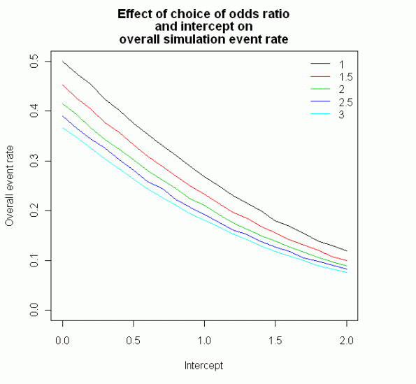
This plot shows how the intercept and odds ratio affect the overall proportion of events per trial:

When you’re happy that the proportion of events is right (with some prior knowledge of the dataset), you can then fit a model and calculate a p value for that model. We use R’s inbuilt function replicate to do this 10,000 times, and count the proportion where it gets it right (i.e. p < 0.05). The proportion of the time that the simulation correctly get's the p < 0.05 is essentially the power of the logistic regression for your number of cases, odds ratio and intercept.

result <-  replicate(
              n = runs,
              expr = {
                  xtest <- rnorm(nn)
                  linpred <- intercept + (xtest * beta)
                  prob <- exp(linpred)/(1 + exp(linpred))
                  runis <- runif(length(xtest),0,1)
                  ytest <- ifelse(runis < prob,1,0)
                  summary(model <- glm(ytest ~ xtest,  family = "binomial"))$coefficients[2,4] < .05
                  }
            )
print(sum(result)/runs)

I checked it against the examples given in Hsieh, 1999.  It seemed to work pretty well calculating the power to be within ~ 1% of the power of the examples given in table II of that paper.

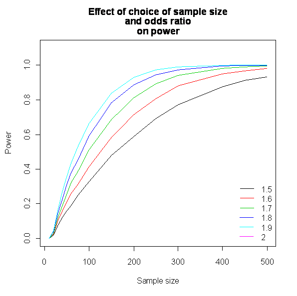
We can do some interesting things with R. I simulated a range of odds ratios and a range of sample sizes. The plot of these looks like this (each line represents an odd ratio):-

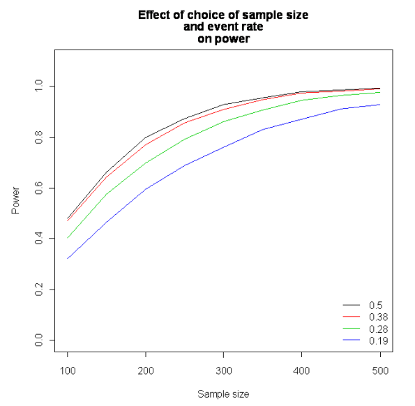
We can also keep the odds ratio constant, but adjust the proportion of events per trial. This looks like this (each line represents an event rate):

As ever, if anyone can spot an error or suggest a simpler way to do this then let me know. I haven’t tested my simulation against any packages which calculate power for logistic regression, but if anyone can it would be great to hear from you.