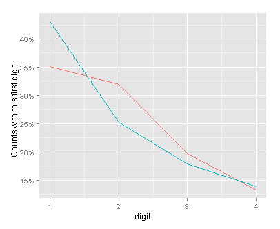
Benford’s Law after converting count data to be in base 5

Firstly, I know nothing about election fraud – this isn’t a serious post. But, I do like to do some simple coding. Ben Goldacre posted on using Benford’s Law to look for evidence of Russian election fraud. Then Richie Cotton did the same, but using R. Commenters on both sites suggested that as the data didn’t span a large order of magnitude, turning it into a lower base (e.g. base 5) may helpful. I’ve no idea if this would be helpful, but the idea of messing around with the data was appealing, so here it is.

The as.binary() function was posted to R-help by Robin Hankin. The code to do the analysis was by Richie Cotton. Putting it all together gives:

So there we have it – with the numerical data in base 5, the observed and expected values are closer together than with the numerical data in base 10. The overall dynamic range is from 1 to 30430 (in base 5).

The data are here. The code you’ll need is:-

 
## repeat the analysis but with base 5
rm(list = ls())
library(reshape)
library(stringr)
library(ggplot2)
russian <- read.csv("Russian observed results - FullData.csv")

as.binary <- function(n,base=2 , r=FALSE){ 
  ## function written by robin hankin
  out <- NULL 
  while(n > 0) { 
    if(r) { 
      out <- c(out , n%%base) 
    } else { 
      out <- c(n%%base , out) 
    } 
    n <- n %/% base 
  } 
  ans <- str_c(out, collapse = "")
  return(ans)
}
russian <- melt(
  russian[, 9:13], 
  variable_name = "candidate"
  )
russian$base_5_value <- apply(as.matrix(russian$value), MARGIN = 1,
                              FUN = as.binary, base = 5)
russian$base_5_value_1st = str_extract(russian$base_5_value, "[123456789]")

first_digit_counts <- as.vector(table(russian$base_5_value_1st))

first_digit_actual_vs_expected <- data.frame(
  digit            = 1:4,
  actual.count     = first_digit_counts,   
  actual.fraction  = first_digit_counts / nrow(russian),
  benford.fraction = log(1 + 1 / (1:4), base = 5)
  )

a_vs_e <- melt(first_digit_actual_vs_expected[, c("digit", "actual.fraction", "benford.fraction")], id.var = "digit")
(fig1_lines <- ggplot(a_vs_e, aes(digit, value, colour = variable)) +
  geom_line() +
  scale_x_continuous(breaks = 1:4) +
  scale_y_continuous(formatter = "percent") +
  ylab("Counts with this first digit") +
  opts(legend.position = "none")
 )

range(as.numeric(russian$base_5_value), na.rm = T)

Machine learning techniques in the biomedical literature

There are relatively few articles published on using machine learning techniques on what many would consider “classical” biomedical study designs (e.g a sample size of 200 and about 10 parameters) and approaches to dealing with . But they may start being published. This is a list to get going with. No all of the article below fit into the above criteria but I’ve kept them here as they’re interesting (at least to me).

This post was motivated by this question on Crossvalidated. I will add to it as I find them or people point them out to me. It’s very short at the moment! Let me know of any broken links.

Articles
Statnikov A, Wang L, Aliferis CF A comprehensive comparison of random forests and support vector machines for microarray-based cancer classification. BMC Bioinformatics. 2008 Jul 22;9:319.

Van Loon K, Guiza F, Meyfroidt G, Aerts JM, Ramon J, Blockeel H, Bruynooghe M, Van Den Berghe G, Berckmans D. Dynamic data analysis and data mining for prediction of clinical stability. Stud Health Technol Inform. 2009;150:590-4.

Luaces O, Taboada F, Albaiceta GM, Domínguez LA, Enríquez P, Bahamonde A; GRECIA Group.Predicting the probability of survival in intensive care unit patients from a small number of variables and training examples.Artif Intell Med. 2009 Jan;45(1):63-76. Epub 2009 Jan 29.

Wu TT, Chen YF, Hastie T, Sobel E, Lange K. Genome-wide association analysis by lasso penalized logistic regression. Bioinformatics. 2009 Mar 15;25(6):714-21. Epub 2009 Jan 28.

Schwaighofer A, Schroeter T, Mika S, Blanchard G. Comb Chem High Throughput Screen. How wrong can we get? A review of machine learning approaches and error bars. 2009 Jun;12(5):453-68.

Huang H, Chanda P, Alonso A, Bader JS, Arking DE. Gene-based tests of association. PLoS Genet. 2011 Jul;7(7):e1002177. Epub 2011 Jul 28.

Liu Z, Shen Y, Ott J. Multilocus association mapping using generalized ridge logistic regression. BMC Bioinformatics. 2011 Sep 29;12:384.

Theses

Hug, Caleb W. Predicting the risk and trajectory of intensive care patients using survival models. 2006 Massachusetts Institute of Technology

Talks / slides / videos:
Victoria Stodden’s slides